
Examples / 06
When the result is not a measurement: weld seams with an ordinal and a nominal response
Not every response is a number. A weld seam is looked at and classified: how much spatter lies next to it, and which defect does the cross-section show? The first answer has an order, the second has none. Here 81 plates are welded at three settings, the spatter is analysed with an ordinal model and the weld defect with a multinomial one, and at the end there is the setting at which a good seam is most likely.
- Design
- 3³ full factorial, 3 plates per setting = 81
- Models
- proportional odds (ordinal), multinomial logit
- Factors
- current, travel speed, shielding gas
- Responses
- 2 with 4 categories each, confirmed with 24 plates
The judgements are simulated. They come from two models we set ourselves — for every plate a category is drawn from the true probabilities. That makes it possible to check at the end whether the analysis finds what is really in there. Every table and chart was computed and drawn by DoEStat.
Step 1 / The question
One seam, two judgements
For a fillet weld on structural steel, a MAG setting is wanted that gives a defect-free seam with little spatter as often as possible. Three settings are free:
| Factor | Unit | low | centre | high |
|---|---|---|---|---|
| Welding current | A | 160 | 200 | 240 |
| Travel speed | cm/min | 30 | 45 | 60 |
| Shielding gas flow | l/min | 8 | 14 | 20 |
Every plate is judged twice: the spatter by eye on a four-step scale, the weld defect in the cross-section. Both responses have four categories — but not of the same kind:
| Response | Kind | Categories |
|---|---|---|
| Spatter | ordinal (ranked) | none < few < moderate < many |
| Weld defect | nominal (no order) | none · porosity · lack of fusion · undercut |
“Few” spatter lies between “none” and “moderate” — the steps are ranked, but the distances between them are unknown; “moderate” does not mean “twice as many as few”. The weld defects, by contrast, are only named: porosity is not “more” than lack of fusion, it has a different cause. This distinction decides the model. In DoEStat it is set in the definition of the response: list the levels, tick “ordered” or not.
Putting a regression on these data as if the categories were the numbers 1 to 4 would be wrong in both cases: the weld defect has no order, the spatter no equal distances. What can be modelled is the probability of each category depending on the setting.
Step 2 / Planning
How many plates does a judgement need?
A category carries less information than a measurement. A single plate only says “porosity” or “no porosity” — the probability behind it only emerges from many. A full factorial with three levels per factor has 27 settings; the question is how often each has to be welded.
The table shows how often the analysis is usable when the whole study is drawn a hundred times from the true models. “Usable” means: the model converges, every category occurs, and no estimate runs off to infinity.
| Plates per setting | Plates in total | Spatter (ordinal): usable | Weld defect (nominal): usable |
|---|---|---|---|
| 1 | 27 | 99% | 24% |
| 2 | 54 | 100% | 81% |
| 3 | 81 | 100% | 96% |
| 4 | 108 | 100% | 97% |
The ordinal model is frugal — it estimates one slope per factor, the same for all steps. The nominal one is not: it estimates separate slopes for each of the three defects, twelve parameters instead of six. With one plate per setting it is unusable in three studies out of four, with two still in one out of five. From three plates per setting it is 96%, and a fourth adds little. The choice is therefore 81 plates.
What “running off to infinity” means is separation: if a rare defect never occurs for a group of settings, its probability there can be pushed arbitrarily close to zero, and the estimate grows without bound. DoEStat reports this in the analysis (“separation suspected”). The problem grows with every additional term — a squared gas term, which suggests itself in a three-level design, leaves only 45 of 100 nominal analyses usable at 81 plates in the same simulation, instead of 96. The model here therefore has main effects only.
This planning calculation is done by the example itself, by repeating the study from the true models. The power analysis in DoEStat covers numeric and binomial responses, not categorical ones with more than two levels.
Step 3 / Runs
81 plates, judged twice
The 81 plates are welded in random order. Only 22 of them are good in the sense of the question — no weld defect and at most a few spatters. Counted by the levels of each factor, the direction shows even before any model:
| Setting | none | porosity | lack of fusion | undercut |
|---|---|---|---|---|
| Welding current 160 A | 10 | 4 | 13 | 0 |
| Welding current 200 A | 14 | 4 | 7 | 2 |
| Welding current 240 A | 10 | 5 | 0 | 12 |
| Travel speed 30 cm/min | 16 | 8 | 1 | 2 |
| Travel speed 45 cm/min | 12 | 3 | 7 | 5 |
| Travel speed 60 cm/min | 6 | 2 | 12 | 7 |
| Shielding gas flow 8 l/min | 9 | 9 | 6 | 3 |
| Shielding gas flow 14 l/min | 11 | 3 | 7 | 6 |
| Shielding gas flow 20 l/min | 14 | 1 | 7 | 5 |
Lack of fusion piles up at low current and fast travel — too little heat, the seam does not fuse with the base metal. Undercuts come with high current. Porosity depends on the shielding gas: frequent at 8 l/min, rare at 20 l/min.
| Setting | none | few | moderate | many |
|---|---|---|---|---|
| Welding current 160 A | 16 | 11 | 0 | 0 |
| Welding current 200 A | 8 | 8 | 7 | 4 |
| Welding current 240 A | 0 | 9 | 7 | 11 |
| Travel speed 30 cm/min | 9 | 11 | 2 | 5 |
| Travel speed 45 cm/min | 7 | 9 | 6 | 5 |
| Travel speed 60 cm/min | 8 | 8 | 6 | 5 |
| Shielding gas flow 8 l/min | 6 | 10 | 3 | 8 |
| Shielding gas flow 14 l/min | 8 | 8 | 5 | 6 |
| Shielding gas flow 20 l/min | 10 | 10 | 6 | 1 |
For the spatter, the current dominates: at 160 A there are never more than a few, at 240 A not a single plate without spatter and two thirds with moderate or many. Little shielding gas makes the arc less steady.
All 81 plates
| Plate | Welding current [A] | Travel speed [cm/min] | Shielding gas flow [l/min] | Spatter | Weld defect |
|---|---|---|---|---|---|
| 1 | 200 | 60 | 14 | moderate | lack of fusion |
| 2 | 240 | 30 | 14 | many | undercut |
| 3 | 240 | 60 | 14 | many | undercut |
| 4 | 240 | 45 | 8 | many | porosity |
| 5 | 240 | 60 | 20 | moderate | undercut |
| 6 | 160 | 30 | 14 | few | none |
| 7 | 160 | 60 | 20 | few | lack of fusion |
| 8 | 240 | 45 | 8 | few | undercut |
| 9 | 200 | 30 | 8 | few | porosity |
| 10 | 240 | 60 | 8 | many | undercut |
| 11 | 240 | 45 | 8 | many | porosity |
| 12 | 160 | 60 | 14 | none | lack of fusion |
| 13 | 160 | 30 | 20 | none | none |
| 14 | 200 | 60 | 8 | none | porosity |
| 15 | 160 | 60 | 8 | none | lack of fusion |
| 16 | 160 | 30 | 8 | none | none |
| 17 | 160 | 30 | 20 | none | none |
| 18 | 240 | 30 | 8 | many | none |
| 19 | 160 | 60 | 14 | none | lack of fusion |
| 20 | 240 | 30 | 20 | few | none |
| 21 | 160 | 60 | 20 | none | lack of fusion |
| 22 | 160 | 45 | 8 | few | lack of fusion |
| 23 | 200 | 60 | 14 | none | none |
| 24 | 240 | 60 | 20 | few | undercut |
| 25 | 160 | 45 | 20 | none | none |
| 26 | 240 | 60 | 14 | few | undercut |
| 27 | 200 | 45 | 20 | many | lack of fusion |
| 28 | 160 | 45 | 14 | none | lack of fusion |
| 29 | 200 | 30 | 8 | few | porosity |
| 30 | 240 | 60 | 20 | moderate | undercut |
| 31 | 200 | 60 | 20 | few | none |
| 32 | 160 | 45 | 14 | none | lack of fusion |
| 33 | 240 | 45 | 14 | few | undercut |
| 34 | 200 | 30 | 14 | few | none |
| 35 | 240 | 60 | 14 | many | none |
| 36 | 240 | 60 | 8 | many | undercut |
| 37 | 240 | 45 | 20 | few | porosity |
| 38 | 240 | 45 | 20 | moderate | none |
| 39 | 160 | 60 | 20 | few | none |
| 40 | 160 | 30 | 8 | none | none |
| 41 | 160 | 30 | 14 | none | porosity |
| 42 | 160 | 45 | 20 | none | none |
| 43 | 200 | 30 | 20 | few | undercut |
| 44 | 200 | 45 | 14 | none | undercut |
| 45 | 200 | 45 | 14 | moderate | none |
| 46 | 240 | 30 | 20 | few | none |
| 47 | 200 | 45 | 20 | moderate | lack of fusion |
| 48 | 240 | 45 | 20 | moderate | undercut |
| 49 | 160 | 60 | 14 | none | lack of fusion |
| 50 | 240 | 45 | 14 | many | none |
| 51 | 160 | 45 | 8 | few | lack of fusion |
| 52 | 240 | 45 | 14 | moderate | undercut |
| 53 | 160 | 45 | 8 | none | none |
| 54 | 200 | 30 | 8 | none | porosity |
| 55 | 200 | 45 | 8 | few | none |
| 56 | 240 | 30 | 20 | moderate | none |
| 57 | 160 | 30 | 8 | few | porosity |
| 58 | 160 | 60 | 8 | few | porosity |
| 59 | 200 | 30 | 20 | none | none |
| 60 | 200 | 45 | 20 | none | none |
| 61 | 200 | 45 | 14 | few | none |
| 62 | 200 | 60 | 8 | many | lack of fusion |
| 63 | 200 | 60 | 8 | moderate | lack of fusion |
| 64 | 240 | 30 | 14 | many | none |
| 65 | 200 | 30 | 14 | moderate | none |
| 66 | 240 | 30 | 8 | few | none |
| 67 | 240 | 30 | 14 | few | porosity |
| 68 | 200 | 60 | 20 | few | none |
| 69 | 160 | 45 | 14 | few | none |
| 70 | 200 | 30 | 14 | many | none |
| 71 | 160 | 30 | 14 | few | porosity |
| 72 | 160 | 45 | 20 | few | lack of fusion |
| 73 | 160 | 30 | 20 | none | lack of fusion |
| 74 | 160 | 60 | 8 | few | lack of fusion |
| 75 | 200 | 60 | 20 | none | lack of fusion |
| 76 | 240 | 60 | 8 | moderate | none |
| 77 | 200 | 60 | 14 | moderate | lack of fusion |
| 78 | 200 | 45 | 8 | moderate | none |
| 79 | 200 | 45 | 8 | many | none |
| 80 | 240 | 30 | 8 | many | porosity |
| 81 | 200 | 30 | 20 | none | none |
Step 4 / Spatter
Ranked steps: the proportional-odds model
For a ranked response DoEStat chooses the cumulative logit model: it describes the probability of reaching at most a given step. One can picture an invisible spatter tendency behind the four steps that the factors shift; three cut-points divide it into the steps. Each factor gets one slope that applies to all three cut-points — hence “proportional odds”.
| Term | Estimate | Std. error | z | p-value | True value |
|---|---|---|---|---|---|
| Welding current | 1.88 | 0.33 | 5.73 | < 0.0001 | 1.50 |
| Travel speed | 0.26 | 0.27 | 0.97 | 0.3342 | 0.30 |
| Shielding gas flow | −0.72 | 0.27 | −2.63 | 0.0085 | −0.80 |
A positive slope pushes the seam towards more spatter. The current acts strongly (z = 5.7), the shielding gas dampens (p = 0.008), the travel speed is not detectable (p = 0.33). The column “True value” is the comparison with the model the data come from — the current is somewhat overestimated, the direction and ranking are right.
| Cut-point | Estimate | Std. error | True value |
|---|---|---|---|
| none | few | −1.39 | 0.32 | −1.00 |
| few | moderate | 0.89 | 0.29 | 0.80 |
| moderate | many | 2.18 | 0.37 | 2.40 |
Does the assumption of equal slopes hold?
The model claims that a factor acts equally strongly at every cut-point. Whether the data support this is checked by the Brant test: it estimates the three cut-points separately and compares the slopes. A small p-value would mean that a factor acts differently between “none” and “few”, say, than between “moderate” and “many” — the multinomial model would then be the more honest choice.
| Term | χ² | df | p-value |
|---|---|---|---|
| Welding current | 0.03 | 2 | 0.9836 |
| Travel speed | 2.07 | 2 | 0.3543 |
| Shielding gas flow | 2.70 | 2 | 0.2594 |
| Overall (omnibus) | 5.19 | 6 | 0.5198 |
No factor objects (jointly p = 0.52). The ordinal model may stay — and for three factors it needs three slopes instead of nine.
| Log-likelihood | without factors | Likelihood-ratio test χ² (df) | p-value | McFadden R² | AIC |
|---|---|---|---|---|---|
| −85.8 | −108.8 | 45.9 (3) | < 0.0001 | 0.211 | 183.7 |
| observed ↓ / predicted → | none | few | moderate | many | Correct |
|---|---|---|---|---|---|
| none | 15 | 9 | 0 | 0 | 15 / 24 |
| few | 9 | 13 | 0 | 6 | 13 / 28 |
| moderate | 0 | 10 | 0 | 4 | 0 / 14 |
| many | 0 | 4 | 0 | 11 | 11 / 15 |
| Accuracy | 48% |
The confusion matrix compares the observed step with the most likely step according to the model. 48% hits sound low, but that is the nature of a probability: at a setting with 45% “few” and 35% “none”, “few” is the best prediction and still often wrong. “Moderate” is never the most likely step — it lies between two neighbours that are each more frequent. What the model separates reliably are the ends: no plate with “no” spatter is predicted as “moderate” or “many”, and vice versa.
Step 5 / Weld defect
Named categories: the multinomial logit
Without an order there is no common scale. The multinomial logit therefore compares each defect separately with a reference category — here “none” — and gives each defect its own slopes. That way the current may prevent lack of fusion and at the same time cause undercuts, without the two cancelling each other out.
| Class against “none” | Term | Estimate | Std. error | p-value | True value |
|---|---|---|---|---|---|
| porosity | Intercept | −1.52 | 0.50 | 0.0021 | −1.20 |
| porosity | Welding current | 0.15 | 0.47 | 0.7435 | 0.00 |
| porosity | Travel speed | −0.47 | 0.51 | 0.3566 | 0.00 |
| porosity | Shielding gas flow | −1.42 | 0.53 | 0.0075 | −1.60 |
| lack of fusion | Intercept | −1.45 | 0.51 | 0.0044 | −1.10 |
| lack of fusion | Welding current | −1.75 | 0.62 | 0.0045 | −2.00 |
| lack of fusion | Travel speed | 1.78 | 0.53 | 0.0009 | 1.50 |
| lack of fusion | Shielding gas flow | −0.04 | 0.44 | 0.9301 | 0.00 |
| undercut | Intercept | −2.20 | 0.75 | 0.0032 | −1.70 |
| undercut | Welding current | 2.35 | 0.83 | 0.0046 | 1.80 |
| undercut | Travel speed | 1.05 | 0.51 | 0.0394 | 1.20 |
| undercut | Shielding gas flow | 0.13 | 0.49 | 0.7863 | 0.00 |
Each defect has its own cause, and the analysis finds it: porosity at the shielding gas (−1.42, true −1.6), lack of fusion at low current and fast travel, undercuts at high current and — more weakly — fast travel. All terms that are zero in the true model stay inconspicuous (p > 0.3).
| Log-likelihood | without factors | Likelihood-ratio test χ² (df) | p-value | McFadden R² | AIC |
|---|---|---|---|---|---|
| −71.2 | −105.8 | 69.3 (9) | < 0.0001 | 0.327 | 166.4 |
| observed ↓ / predicted → | none | porosity | lack of fusion | undercut | Correct |
|---|---|---|---|---|---|
| none | 18 | 4 | 8 | 4 | 18 / 34 |
| porosity | 3 | 7 | 2 | 1 | 7 / 13 |
| lack of fusion | 3 | 0 | 17 | 0 | 17 / 20 |
| undercut | 3 | 1 | 0 | 10 | 10 / 14 |
| Accuracy | 64% |
The model recognises lack of fusion and undercuts best — they have clear, opposing causes. The defect-free seam is the hardest to predict: it is what remains when none of the three defects occurs, and so it has no cause of its own.
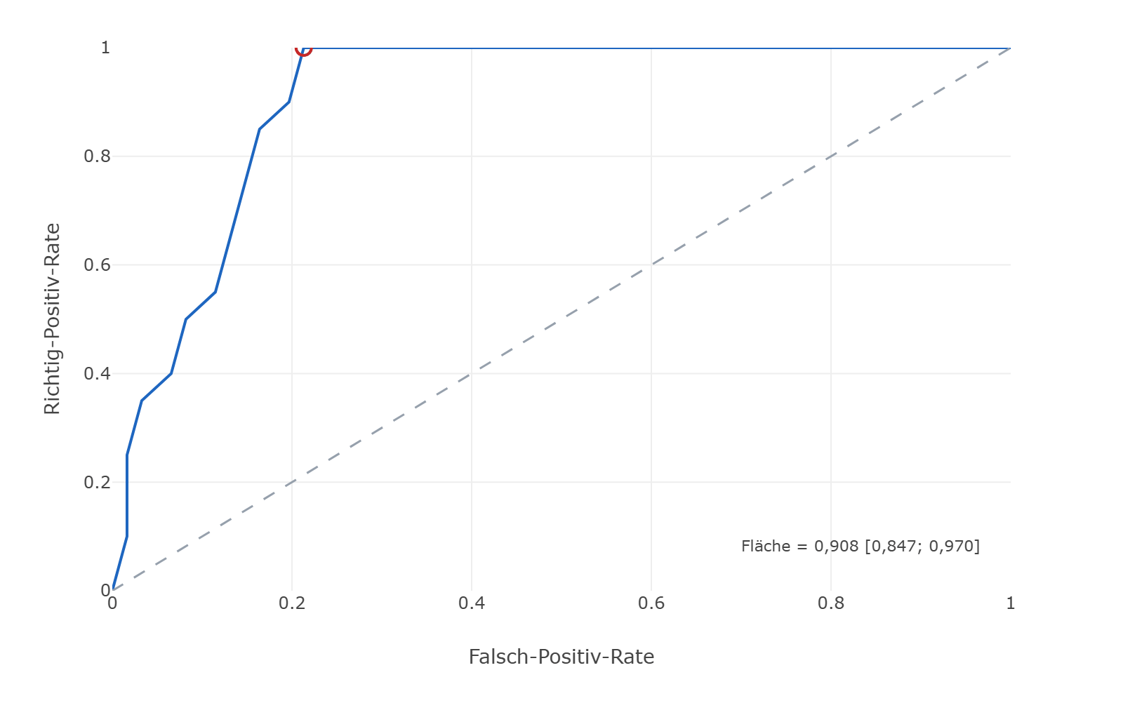
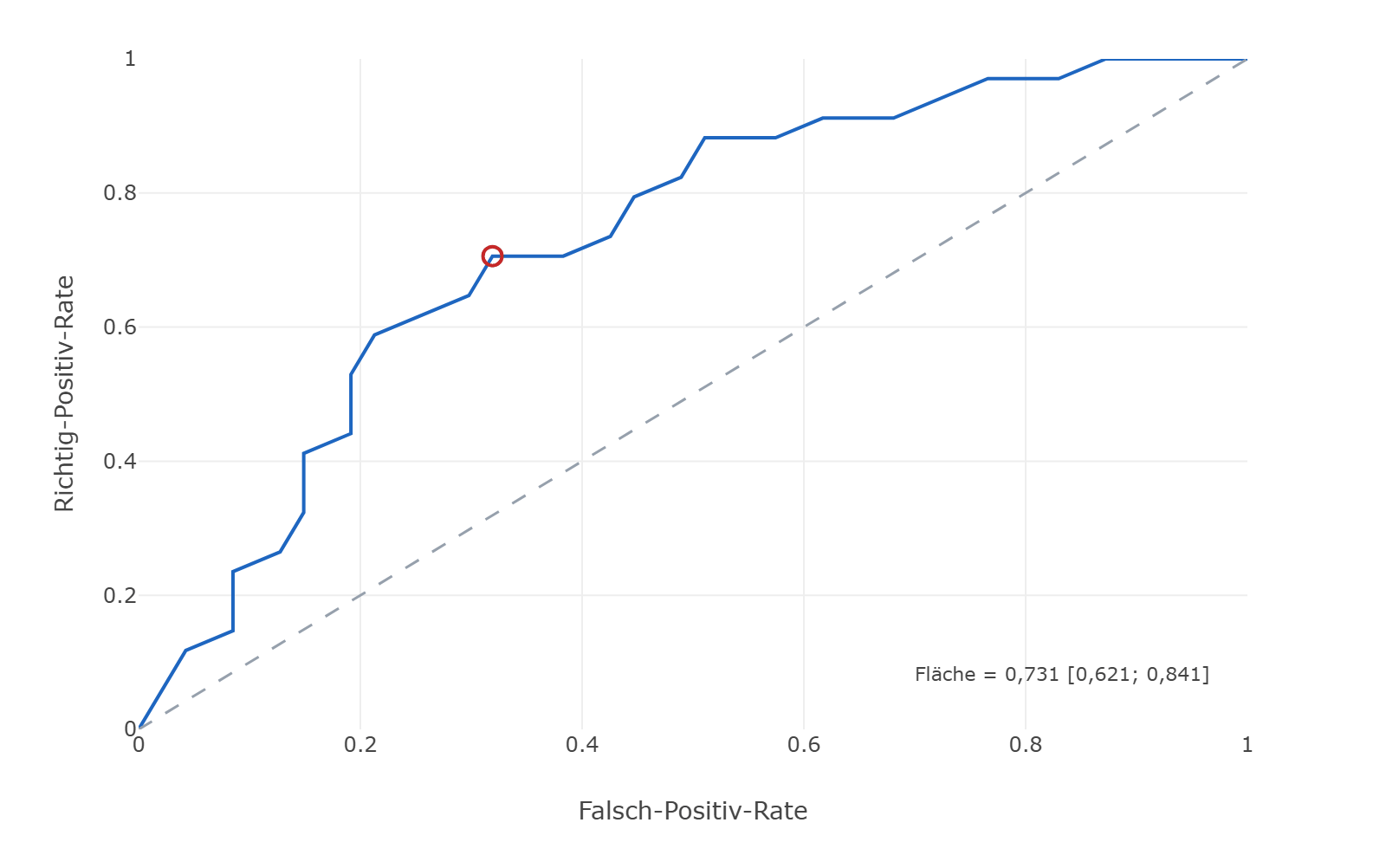
| Class | Count | AUC | 95% interval |
|---|---|---|---|
| none | 34 | 0.731 | 0.621 … 0.841 |
| porosity | 13 | 0.799 | 0.660 … 0.938 |
| lack of fusion | 20 | 0.908 | 0.847 … 0.970 |
| undercut | 14 | 0.900 | 0.810 … 0.989 |
The ROC curves that DoEStat draws for each category against all others show the same: the area under the curve is 0.91 for lack of fusion and 0.73 for the defect-free seam.
Step 6 / Process window
Where a good seam is most likely
The probability profiler shows, for each category, how its probability changes when one factor is moved and the others are held. The four curves in a column add up to one everywhere. In DoEStat the lines are dragged with the mouse and both responses are seen at once.
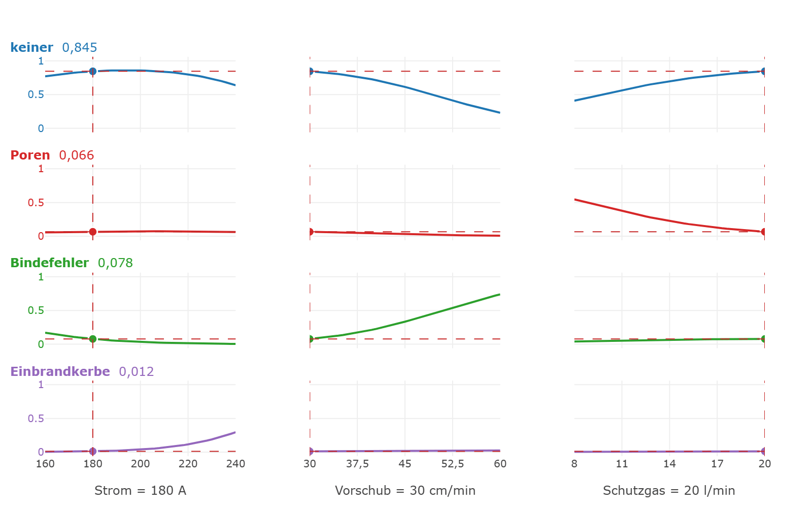
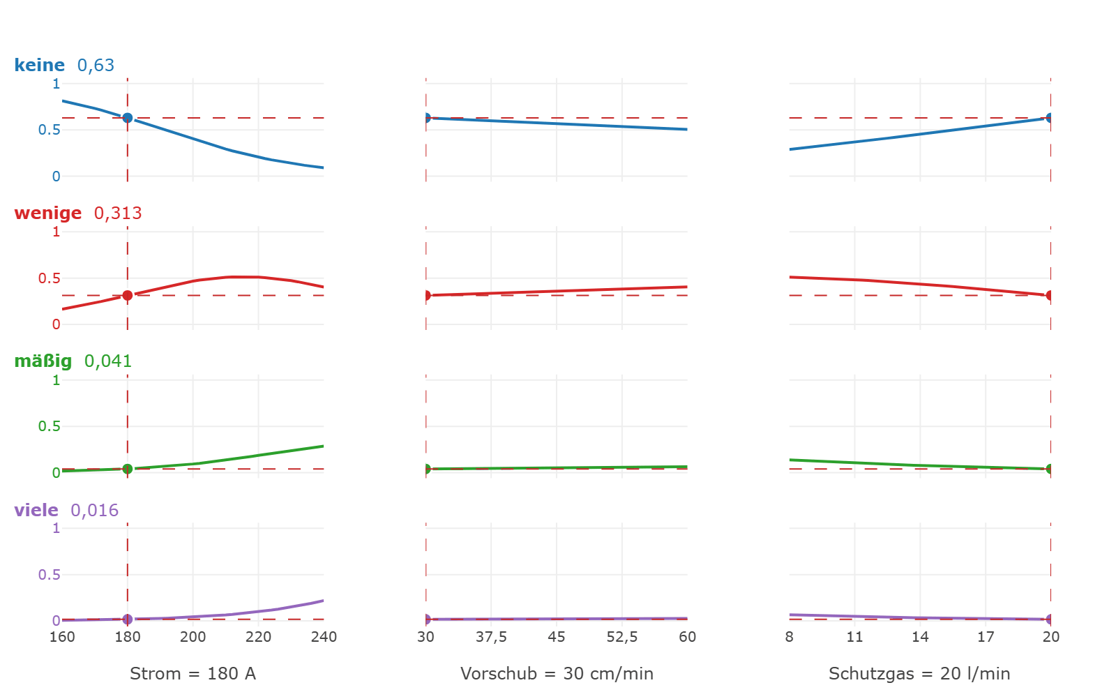
The profilers stand at the setting at which a good plate — no weld defect, at most a few spatters — is most likely. It was found as the product of the two probabilities over a grid of the region:
| Factor | Setting | Unit | coded |
|---|---|---|---|
| Welding current | 180 | A | −0.50 |
| Travel speed | 30 | cm/min | −1.00 |
| Shielding gas flow | 20 | l/min | 1.00 |
The current lies in the lower quarter of the range: more current brings spatter and undercuts, less brings lack of fusion. Travel speed and shielding gas sit on the edge of the region — welding slowly with plenty of gas is simply better here. Anyone searching beyond that leaves the region studied; the model knows nothing there.
Step 7 / Confirmation
24 plates at the chosen setting
A probability is not confirmed with one plate. At the chosen setting 24 plates are welded and judged as in the study:
| Response | Category | Model prediction | True probability | Confirmation (24 plates) |
|---|---|---|---|---|
| Spatter | none | 63% | 70% | 18 |
| few | 31% | 23% | 5 | |
| moderate | 4% | 5% | 1 | |
| many | 2% | 1% | 0 | |
| Weld defect | none | 84% | 78% | 19 |
| porosity | 7% | 5% | 2 | |
| lack of fusion | 8% | 16% | 3 | |
| undercut | 1% | 2% | 0 |
Result: 18 of the 24 plates are good (75%) — in the study it was 22 of 81 (27%). The model had promised 80%; the truth is 73%. The gap is typical: whoever picks the best of all settings also picks the one at which the model happens to be too optimistic. Most clearly for lack of fusion — the model expects 8%, the truth is 16%, and 3 of 24 were observed.
Summing up
What the right scale achieved
Two responses that cannot be measured, only classified, and for each the model that fits its kind. The ordinal model uses the order of the spatter steps and makes do with three slopes; the Brant test confirmed that this is enough. The multinomial model gives each weld defect its own cause — and that was exactly what was needed, because the current prevents one defect and causes another.
The price is the number of plates. Categorical data need replicates, and the nominal model needs more than the ordinal one. The planning calculation beforehand showed that 54 plates would have led to no usable result in one study out of five, and that an obvious squared term makes matters worse.
Against the truth: all factors that act in the true model are found, with the right sign; all that do not act stay inconspicuous. The estimates deviate from the truth by up to a little over half a logit — with 81 plates and one judgement each, that is the precision one can expect. And the confirmation shows that the probability at the best setting is somewhat overestimated: anyone who has to make a commitment takes the result of the confirmation plates, not the prediction.
Project files
Run it yourself
The example ships with DoEStat as a project: Help ▸ Open sample project ▸ Other ▸ “Categorical responses: weld seam”, once with the data only (with the full quadratic model a three-level design is made for) and once with the finished analysis (main effects). The same files can be downloaded here.
- Project with the dataschweissnaht-kategorial-daten.doejson
- Project with the finished analysisschweissnaht-kategorial-auswertung.doejson
Try DoEStat for free
30 days, the full feature set, no payment details. We send the download link by e-mail, usually on the next business day.