
Examples / 05
Simulation instead of a test rig: a heat sink designed with Gaussian processes
When the runs take place in a simulation program, what makes a good design changes. There is no scatter that would need replicates, but every run costs computing time. Here five settings of a heat sink are spread over the whole region in 40 simulations, a Gaussian process (kriging) learns three responses from them, and desirability finds the sweet spot. Three prototypes built and measured in the wind tunnel show at the end how far the simulation can be trusted.
- Design
- MaxPro, 40 simulations + 2 for sharpening
- Model
- Gaussian process, Matérn 5/2
- Factors
- 5 geometry and flow settings
- Responses
- 3, confirmed with 3 prototypes
Simulator and prototypes are emulated. Instead of a flow solver, a model built from textbook formulas for fin efficiency, heat transfer and pressure drop does the computing — not linear, without scatter, like a real simulator. The wind-tunnel measurements are the same formulas with a systematic offset and measurement scatter. That makes it possible to check at the end what the Gaussian process has learned. Every table and chart was computed and drawn by DoEStat.
Step 1 / The question
One heat sink, three limits
A power module with a 100 × 100 mm footprint is to be cooled by an aluminium finned heat sink with a fan blowing through it. The design is done in a thermal simulation; one run takes a good quarter of an hour, 40 runs fit into one night. Three quantities decide the design:
- Thermal resistance from the module to the air — to be minimised, at most 0.35 K/W
- Pressure drop across the heat sink — to be minimised, at most 60 Pa, or the fan cannot cope
- Mass — to be minimised, at most 450 g
The three pull against each other: tall, closely spaced fins cool well but cost mass and pressure; more air cools better and costs pressure too. Five settings are free:
| Factor | Unit | from | to |
|---|---|---|---|
| Fin height | mm | 20.0 | 60.0 |
| Fin thickness | mm | 1.00 | 3.00 |
| Fin gap | mm | 2.00 | 8.00 |
| Air flow | m³/h | 10.0 | 40.0 |
| Base thickness | mm | 4.0 | 12.0 |
Step 2 / Design
40 points that fill the region
A classical design is the wrong choice here. A central composite design puts its points on corners, faces and the centre, so it knows only three levels per factor, and it replicates the centre to estimate scatter. A simulator, however, returns the same number for the same input every time; every replicate would be wasted computing time. And whether the surfaces behave like a second-order polynomial nobody knows beforehand.
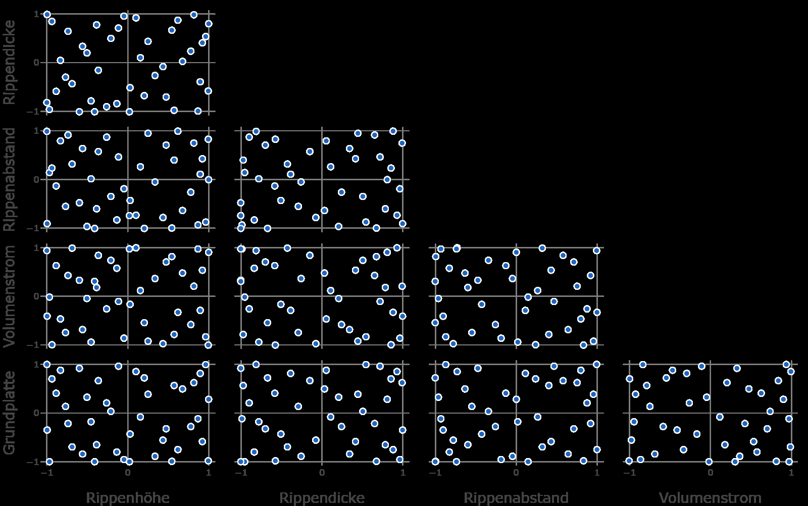
A space-filling design spreads the runs evenly over the interior instead. DoEStat offers several families for this. The one chosen is MaxPro (Joseph, Gul and Ba, 2015): the points are well spread not only in the five-dimensional region but also in every projection onto two, three or four factors. That matters as soon as a factor turns out to have no effect — then points fall onto each other in other designs, and the information shrinks.
| Metric | MaxPro, 40 (chosen) | Sphere packing, 40 | Maximin Latin hypercube, 40 | Central composite, 43 |
|---|---|---|---|---|
| MaxPro criterion ψ (projections, smaller is better) | 23.06 | ∞ | 144.00 | ∞ |
| Smallest distance between two points (unit cube) | 0.425 | 0.866 | 0.297 | 0.500 |
| Coverage radius (largest gap) | 0.720 | 0.751 | 0.713 | 0.642 |
| Largest column correlation |r| | 0.108 | 0.027 | 0.205 | 0.000 |
| Distinct levels per factor | 40 | 7 | 40 | 3 |
The design evaluation shows the difference. Sphere packing keeps the largest minimum distance in the full region but uses only seven distinct values per factor for it. The central composite design has three. In both, points coincide in a projection, and the MaxPro criterion is infinite. MaxPro and the Latin hypercube have 40 distinct values per factor, but MaxPro spreads them far better in the projections.
Step 3 / Simulation
One night of computing
The design goes to the simulation as a table, and the results come back into the same table. In DoEStat a simulator can also be connected directly: a Python script receives the settings of a run and returns the responses; the runs then fill the data table without a detour through files.
What stands out in the results is their range: the thermal resistance runs from 0.20 to 1.10 K/W, the mass from 200 to almost 1,200 g, the pressure drop from under one to 70 Pa. The physics behind it is not linear — the efficiency of a fin follows a hyperbolic tangent, the pressure drop the square of the flow velocity.
And none of the 40 simulations keeps all three limits at once. Anyone simply taking the best run from the table would have nothing usable. The sweet spot lies between the points — where only a model can look.
All simulations
| Run | Fin height [mm] | Fin thickness [mm] | Fin gap [mm] | Air flow [m³/h] | Base thickness [mm] | Thermal resistance [K/W] | Pressure drop [Pa] | Mass [g] |
|---|---|---|---|---|---|---|---|---|
| 1 | 60.0 | 2.81 | 5.01 | 38.6 | 9.1 | 0.3829 | 10.92 | 858.1 |
| 2 | 22.3 | 1.42 | 4.62 | 34.5 | 9.6 | 0.5394 | 41.92 | 408.2 |
| 3 | 37.7 | 2.72 | 6.41 | 23.4 | 11.9 | 0.6583 | 8.06 | 643.2 |
| 4 | 20.6 | 1.05 | 5.44 | 24.8 | 4.0 | 0.7073 | 20.92 | 202.9 |
| 5 | 53.5 | 2.03 | 3.10 | 32.2 | 10.0 | 0.2985 | 14.01 | 859.9 |
| 6 | 44.1 | 1.33 | 2.00 | 16.9 | 10.9 | 0.2756 | 11.18 | 779.2 |
| 7 | 28.0 | 1.00 | 3.58 | 30.0 | 11.7 | 0.4142 | 22.43 | 486.6 |
| 8 | 45.0 | 2.45 | 7.87 | 11.2 | 9.5 | 0.8111 | 1.20 | 568.8 |
| 9 | 57.9 | 1.62 | 5.34 | 20.7 | 11.3 | 0.4470 | 2.66 | 686.8 |
| 10 | 20.0 | 1.19 | 7.99 | 39.1 | 12.0 | 0.7715 | 45.34 | 399.6 |
| 11 | 56.3 | 2.99 | 7.26 | 28.1 | 10.5 | 0.5552 | 5.00 | 759.9 |
| 12 | 29.9 | 2.21 | 2.12 | 24.4 | 9.3 | 0.3492 | 45.68 | 672.3 |
| 13 | 51.5 | 1.03 | 6.22 | 13.3 | 10.3 | 0.5679 | 1.15 | 487.1 |
| 14 | 59.9 | 1.43 | 7.50 | 10.0 | 4.1 | 0.6439 | 0.51 | 387.9 |
| 15 | 37.3 | 1.17 | 2.52 | 33.7 | 4.8 | 0.2871 | 26.32 | 455.9 |
| 16 | 28.8 | 2.34 | 6.93 | 14.8 | 4.6 | 0.9127 | 4.96 | 335.4 |
| 17 | 43.1 | 2.11 | 5.80 | 26.8 | 7.7 | 0.5348 | 7.57 | 536.1 |
| 18 | 50.9 | 2.68 | 2.02 | 37.3 | 4.0 | 0.2506 | 48.54 | 907.6 |
| 19 | 42.0 | 2.93 | 2.81 | 40.0 | 11.4 | 0.3121 | 48.23 | 903.5 |
| 20 | 32.7 | 1.85 | 6.74 | 37.7 | 10.7 | 0.5909 | 20.32 | 491.3 |
| 21 | 23.4 | 2.06 | 7.40 | 18.0 | 11.5 | 0.9686 | 9.64 | 458.5 |
| 22 | 20.1 | 3.00 | 2.29 | 18.9 | 6.6 | 0.5347 | 69.66 | 492.3 |
| 23 | 55.6 | 2.24 | 4.23 | 16.3 | 6.9 | 0.4377 | 3.00 | 728.2 |
| 24 | 26.2 | 1.58 | 5.97 | 39.9 | 5.2 | 0.5822 | 35.18 | 297.6 |
| 25 | 48.7 | 1.93 | 2.67 | 10.4 | 5.8 | 0.3841 | 3.64 | 721.9 |
| 26 | 32.3 | 2.79 | 3.21 | 27.8 | 5.4 | 0.4426 | 32.31 | 563.8 |
| 27 | 24.6 | 1.71 | 3.36 | 13.9 | 8.5 | 0.5933 | 10.66 | 462.7 |
| 28 | 40.6 | 1.50 | 3.72 | 22.6 | 6.3 | 0.4134 | 8.20 | 495.0 |
| 29 | 49.5 | 1.30 | 7.14 | 35.6 | 6.7 | 0.5158 | 6.95 | 402.1 |
| 30 | 25.2 | 2.65 | 7.76 | 31.5 | 7.1 | 0.8141 | 26.15 | 379.8 |
| 31 | 58.4 | 2.42 | 6.30 | 33.1 | 5.7 | 0.4674 | 6.29 | 618.1 |
| 32 | 39.1 | 2.97 | 4.44 | 12.1 | 4.2 | 0.6439 | 3.77 | 553.9 |
| 33 | 35.8 | 2.51 | 3.97 | 36.1 | 8.1 | 0.4220 | 30.08 | 609.0 |
| 34 | 52.4 | 2.88 | 8.00 | 20.1 | 5.0 | 0.6781 | 2.78 | 539.6 |
| 35 | 59.3 | 2.55 | 2.39 | 12.5 | 12.0 | 0.3273 | 5.30 | 1169.1 |
| 36 | 34.8 | 1.10 | 7.63 | 21.2 | 8.8 | 0.7349 | 4.76 | 366.2 |
| 37 | 30.9 | 1.22 | 5.06 | 10.9 | 7.3 | 0.6988 | 2.60 | 367.4 |
| 38 | 21.3 | 2.86 | 5.72 | 10.1 | 10.8 | 1.1017 | 5.98 | 494.0 |
| 39 | 57.4 | 1.01 | 2.21 | 39.6 | 7.5 | 0.2047 | 18.93 | 701.2 |
| 40 | 46.7 | 1.75 | 4.87 | 30.5 | 4.4 | 0.4362 | 8.75 | 469.3 |
| 41 | 31.8 | 1.00 | 2.00 | 29.6 | 4.0 | 0.2724 | 35.64 | 400.0 |
| 42 | 40.4 | 1.00 | 2.79 | 39.7 | 4.0 | 0.2811 | 24.58 | 404.0 |
The last two rows are the runs from sharpening (step 6).
Step 4 / Gaussian process
A model that passes through every point
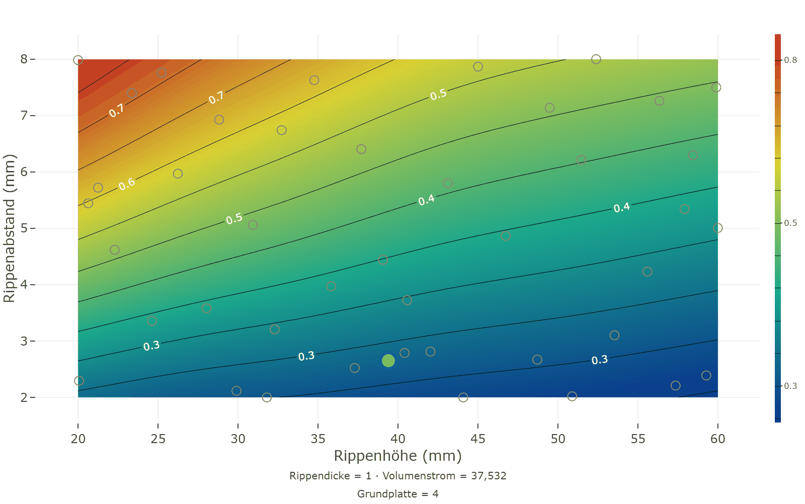
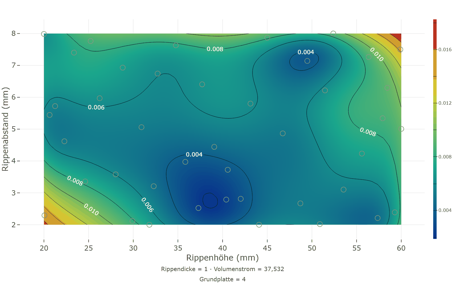
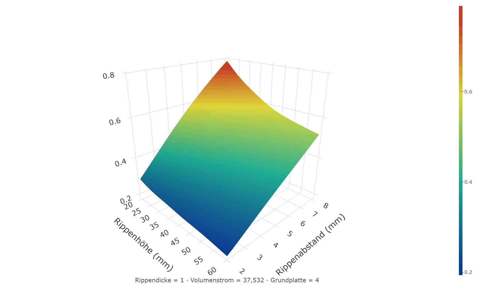
For simulation data one chooses the modelling strategy kriging in DoEStat. A Gaussian process assumes no polynomial. It assumes that settings close to each other give similar results, and estimates from the data how fast that similarity fades with distance — for each factor separately. Because the simulator does not scatter, the surface passes exactly through every computed point. In between it predicts not only a value but also how sure it is.
| Response | Correlation function | Process standard deviation σ | LOO RMSE | Q² (leave-one-out) | Quadratic polynomial: pred. R² |
|---|---|---|---|---|---|
| Thermal resistance [K/W] | Matérn 5/2, one length scale per factor | 0.750 | 0.0182 | 0.9922 | 0.9774 |
| Pressure drop [Pa] | Matérn 5/2, one length scale per factor | 60.5 | 5.02 | 0.9093 | 0.7936 |
| Mass [g] | Matérn 5/2, one length scale per factor | 2061 | 2.71 | 0.9998 | 0.9885 |
For an interpolator, quality is not measured with R² — that would always be 1. Instead every run is left out once and predicted from the others (leave-one-out). Q² is the share of the variation these predictions explain. For comparison, the table shows what a quadratic polynomial achieves on the same data in the same test.
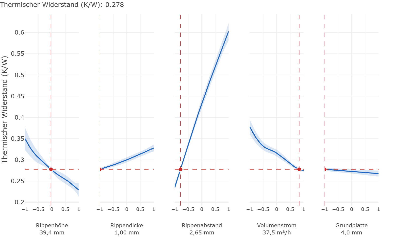
What the process has learned about the factors
The estimated length scales say over what distance (in coded units; the range is 2 wide) a response changes noticeably along a factor. A small number means sensitive. A very large one means the surface is flat in that direction — the factor has no effect.
| Factor | Thermal resistance [K/W] | Pressure drop [Pa] | Mass [g] |
|---|---|---|---|
| Fin height | 3.46 | 2.25 | 9.29 |
| Fin thickness | 15.38 | 7.20 | 10.56 |
| Fin gap | 5.95 | 1.86 | 6.44 |
| Air flow | 3.69 | 4.01 | 1000.00 |
| Base thickness | 205.68 | 1000.00 | 51.83 |
The physics can be recognised in it without anyone having specified it: the base thickness hardly matters for pressure drop and thermal resistance, but very much for the mass. The air flow acts on heat and pressure and does not affect the mass. The importance per factor makes this tangible as a share of the surface's variation:
| Factor | Thermal resistance: main effect | Thermal resistance: total | Pressure drop: main effect | Pressure drop: total | Mass: main effect | Mass: total |
|---|---|---|---|---|---|---|
| Fin height | 24.9% | 28.2% | 31.1% | 43.0% | 36.2% | 40.0% |
| Fin thickness | 1.6% | 1.9% | 3.0% | 5.8% | 17.9% | 19.8% |
| Fin gap | 55.4% | 57.8% | 21.9% | 31.7% | 26.8% | 29.4% |
| Air flow | 14.0% | 16.2% | 26.5% | 36.8% | 0.0% | 0.0% |
| Base thickness | 0.0% | 0.0% | 0.0% | 0.0% | 15.0% | 15.0% |
“Main effect” is the share a factor explains on its own; “total” includes its interplay with the others. For the pressure drop, “total” lies well above the main effect: fin height, fin gap and air flow act together there on the flow velocity. The values are Monte Carlo estimates over the region and scatter by a few percentage points: they are good enough for the ranking of the factors, not for the decimal place.
Step 5 / Diagnostics
How far does the model carry?
An interpolator has no residuals in the usual sense — at the design points it hits exactly. Diagnostics therefore work through the leave-one-out predictions: for every run the deviation of the prediction from the other runs, divided by the standard error the process gives itself for it. If that self-assessment is right, these standardised residuals lie around zero like a standard normal distribution, with only about one value in twenty beyond ±2.
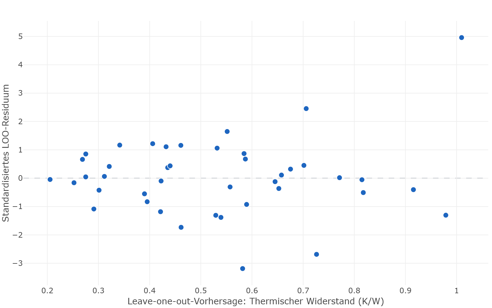
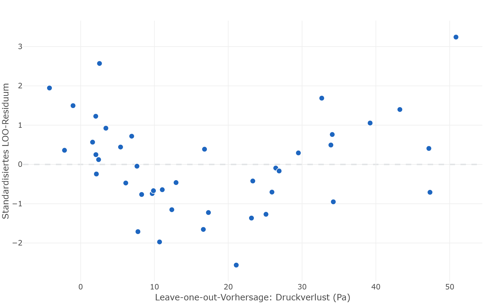
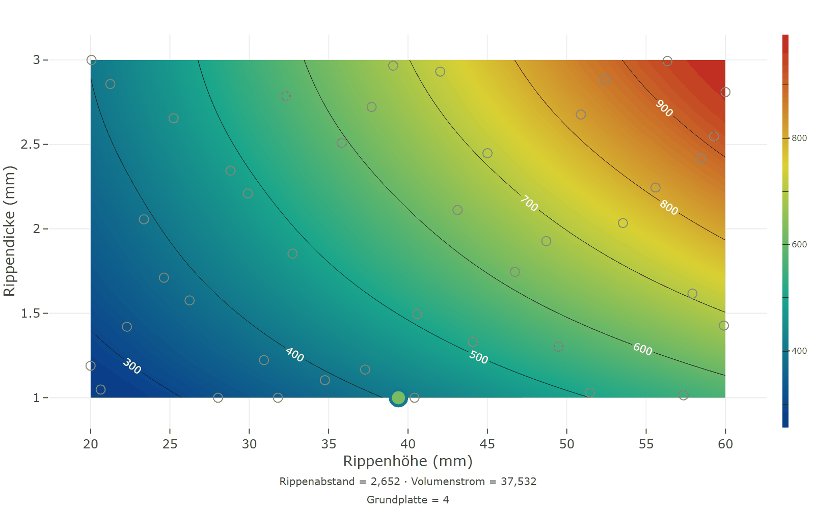
It is not quite right. For the thermal resistance, four of the 42 values lie beyond ±2, one at almost 5; for the pressure drop there are three. The largest of each belongs to an extreme of the design: run 38 has the highest thermal resistance at 1.10 K/W (short fins, wide gap, little air), run 22 the highest pressure drop at 70 Pa — the only one above the limit. Leaving out such a run forces the process to extrapolate into a corner, and there it underestimates its uncertainty.
Two things follow. First, the emulator's band is a lower bound of the uncertainty, not its measure — at the edge of the region in particular. Second, the sweet spot lies far from these corners, in a region the design covers well. Whether the emulator is right there can be checked directly, and that happens in step 6. For the pressure drop, there is also the fact that some predictions in the lower range fall below zero — physically impossible. It is the hardest of the three responses: it grows with the square of the velocity and has its steepest slopes exactly where things get interesting.
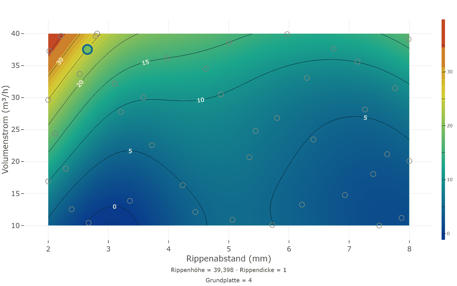
Pressure drop and mass in a cut
Step 6 / Sweet spot
Three limits, one window
Desirability translates every response into a number between 0 (at the limit) and 1 (as good as needed) and looks for the setting at which the weighted mean is largest. Thermal resistance counts three times, pressure drop twice and mass once. The optimisation runs directly on the surfaces of the Gaussian process.
Sharpen first, then build
An optimum on an emulator is a prediction. Before anything is built, the simulator is run at exactly this setting — that costs a quarter of an hour and tells whether the emulator is right there. If it is off, the run joins the data, the process is refitted, and the search starts again. Here two additional simulations were needed for that:
| Round | Overall desirability D | Thermal resistance: emulator ± SE | Thermal resistance: simulation | Pressure drop: emulator ± SE | Pressure drop: simulation | Mass: emulator ± SE | Mass: simulation |
|---|---|---|---|---|---|---|---|
| 1 | 0.398 | 0.2702 ± 0.0063 | 0.2724 | 31.85 ± 2.43 | 35.64 | 401.0 ± 3.2 | 400.0 |
| 2 | 0.403 | 0.2747 ± 0.0069 | 0.2811 | 25.96 ± 1.93 | 24.58 | 406.6 ± 1.4 | 404.0 |
| 3 | 0.397 | 0.2779 ± 0.0020 | 0.2792 | 24.89 ± 0.28 | 24.86 | 407.6 ± 0.2 | 407.0 |
In the first round the pressure drop came out 3.8 Pa above the prediction — a good one and a half standard errors, not surprising in this steep region. With the new point, the optimum moves to more air and a slightly wider fin gap. After the third round, emulator and simulator agree to within one per cent; the search is complete.
| Factor | Setting | Unit | coded |
|---|---|---|---|
| Fin height | 39.40 | mm | −0.03 |
| Fin thickness | 1.000 | mm | −1.00 |
| Fin gap | 2.652 | mm | −0.78 |
| Air flow | 37.53 | m³/h | 0.84 |
| Base thickness | 4.00 | mm | −1.00 |
| Response | Goal | Emulator prediction | Emulator 95% band | Desirability d | Simulation at the setting |
|---|---|---|---|---|---|
| Thermal resistance [K/W] | minimise, at most 0.35 | 0.2779 | 0.2740 … 0.2818 | 0.361 | 0.2792 |
| Pressure drop [Pa] | minimise, at most 60 | 24.89 | 24.34 … 25.44 | 0.702 | 24.86 |
| Mass [g] | minimise, at most 450 | 407.6 | 407.2 … 408.1 | 0.170 | 407.0 |
| Overall desirability D | 0.397 |
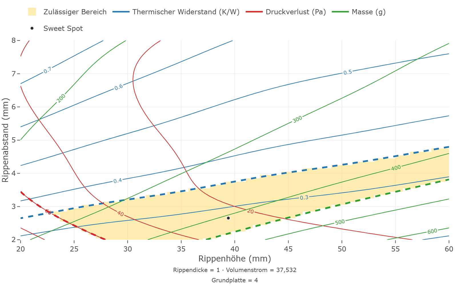
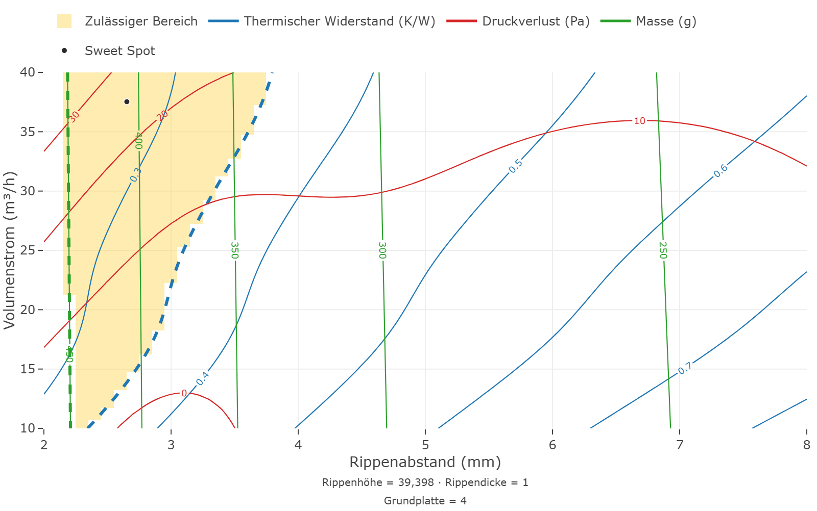
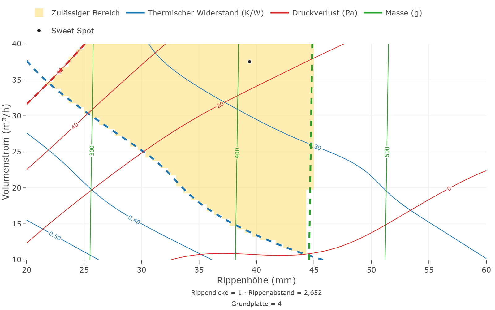
The sweet spot has 1 mm thin fins and a 4 mm base — both at their lower limit, because they only cost mass and hardly cool. The 28 fins stand 2.7 mm apart and are 39 mm tall, and the fan delivers 37.5 m³/h. The lowest individual desirability belongs to the mass (0.17): every millimetre of fin height that lowers the thermal resistance adds aluminium. What binds the overall result, though, is the thermal resistance — it counts three times, so DoEStat names it at the optimum as the goal holding D down the most.
All three responses in one picture
The overlaid view shows the latitude around the sweet spot: the contour lines of every response in its colour, the limits as heavy dashed lines, and shaded the region where all three are kept.
Where the next simulation would go
Anyone who wants to keep computing gets two suggestions from the Gaussian process: the point where it is least sure, and the point most likely to push the thermal resistance below the best so far (expected improvement). Both lie in corners of the region — the first because least is known there, the second because it looks only at the thermal resistance and knows nothing of pressure and mass. For the design, desirability therefore remains decisive.
| Suggestion | Fin height [mm] | Fin thickness [mm] | Fin gap [mm] | Air flow [m³/h] | Base thickness [mm] | Prediction | Standard error | Criterion |
|---|---|---|---|---|---|---|---|---|
| Largest uncertainty | 20.0 | 1.00 | 8.00 | 10.0 | 4.0 | 1.2036 | 0.0250 | max. standard error: 0.0250 |
| Largest expected improvement | 60.0 | 1.00 | 2.00 | 40.0 | 12.0 | 0.1804 | 0.0062 | expected improvement (EI): 0.0243 |
Step 7 / Validation
Three prototypes in the wind tunnel
The emulator reproduces what the simulator computes. Whether the simulator matches reality is a different question, and only an experiment answers it. Three heat sinks are milled to the sweet-spot geometry and measured in the wind tunnel at 37.5 m³/h:
| Response | Simulation | Prototype 1 | Prototype 2 | Prototype 3 | Measured mean | Deviation | Limit |
|---|---|---|---|---|---|---|---|
| Thermal resistance [K/W] | 0.279 | 0.287 | 0.295 | 0.305 | 0.296 | +5.9% | ≤ 0.35 |
| Pressure drop [Pa] | 24.9 | 25.1 | 28.7 | 26.1 | 26.6 | +7.1% | ≤ 60 |
| Mass [g] | 407 | 408 | 406 | 406 | 407 | −0.1% | ≤ 450 |
Result: all three limits are kept on all three prototypes. The simulation is, however, measurably optimistic: the thermal resistance is 6% higher, the pressure drop 7% — the contact resistance under the module and the roughness of the milled channels are in no simulation model. The mass is right. The margin to the limit that desirability left was therefore needed.
Summing up
What the simulation achieved
42 simulations and three prototypes for five factors and three responses. A prototype programme answering the same question in the wind tunnel would have needed 43 milled heat sinks with a central composite design — and with three levels per factor would have captured the curvature of the pressure drop only roughly.
The space-filling design gave the Gaussian process the information it needs: many distinct values per factor and good projections, so that two practically inactive directions cost nothing. From that, the process recognised on its own which factor counts for which response, and stated where it is sure. Sharpening cost two quarter-hours of computing and brought the prediction at the sweet spot from “roughly” to “within one per cent”.
Against the truth: here the simulator is the truth, and the column “Simulation at the setting” in the optimisation table shows it: at the sweet spot the emulator is off by no more than one per cent for any response. What the prototypes show in addition no emulator can learn — the gap between simulation model and reality. For that, confirmation on the real part remains indispensable.
Project files
Run it yourself
The example ships with DoEStat as a project: Help ▸ Open sample project ▸ Other ▸ “Simulation with a Gaussian process: heat sink”, once with the data only and once with the finished analysis. The same files can be downloaded here.
- Project with the datakuehlkoerper-simulation-daten.doejson
- Project with the finished analysiskuehlkoerper-simulation-auswertung.doejson
Back: from screening to a response surface Next: categorical responses
Try DoEStat for free
30 days, the full feature set, no payment details. We send the download link by e-mail, usually on the next business day.